 |
 |
|
 |
||
| Issue 24 | Spring 1999 | |
 |
 |
|
 |
||
| Issue 24 | Spring 1999 | |
Social Research Update is published quarterly by the Department of Sociology, University of Surrey, Guildford GU2 7XH, England. Subscriptions for the hardcopy version are free to researchers with addresses in the UK. Apply by email to sru@soc.surrey.ac.uk.
Optimal Matching Analysis
Tak Wing Chan is a lecturer in Sociology at the University of Surrey. His research interests include social stratification and the life course. His most recent publication is ‘Revolving Doors Reexamined: Occupational Sex Segregation Over the Life Course’, American Sociological Review, 1999, vol.64, pp.86-96.
Email: tw.chan@soc.surrey.ac.uk
Many interesting sociological questions are about process: how do observed social regularities come about? For example, mobility researchers have established that there is a cross-nationally common and over-time persistent mobility pattern, in which people from advantaged class background enjoy better relative mobility chances (Erikson and Goldthorpe 1992). This is an important finding, but we may further ask: how does this pattern come about? Bearing in mind that social mobility is for many people a circuitous process, it is important to ask: how does the multifaceted career process - job-changing, promotion, going into and out of the labour market, etc. - allocate people to different positions in the class structure, in a way which ultimately produces the observed mobility regime.
Clearly, to address questions about social process, we need both longitudinal data relevant to the process of interest and technical tools to analyse those data. Longitudinal data are available (the British Household Panel Study is a prime source for the UK), and we do have a range of analytical tools at our disposal (Dale and Davis 1994).
Of the various tools for longitudinal data analysis, event history models are probably most useful (Blossfeld and Rohwer 1995). They allow the researchers to test how the transition rate of moving from one state (e.g. unemployed) to another (employed) is affected by other variables. Researchers can include previous (employment) history as a covariate. They can also include predictors which measure what is happening in other life domains (e.g. education, family), thus helping us understand the interweaving of multiple processes (see e.g. Blossfeld 1995).
However, event history models invariably consider one transition at a time. If the process in question is repeatable - as in the case when someone moves from being unemployed to employed, back to unemployment, and then finds a job again - the researcher will have to model each transition separately, with the covariates suitably updated each time. This is reasonable for many purposes. But in some cases, we may want to consider the whole sequence of multiple transitions simultaneously, because we want to have a sense of how the individual steps fit together, or because we think that the sequence taken as a whole tells us something important. If this is the case, optimal matching analysis (also known as optimal alignment, hereafter as OMA) is a potentially useful tool.
OMA is a family of procedures that takes into account the full complexity of sequence data. The objective is to identify a typology of sequences empirically. It was developed by, among others, molecular biologists who study protein or DNA sequences. Biologists often wish to find out how different a particular DNA sequence is from other sequences. Knowing this will help them reconstruct the evolutionary tree. There are of course other applications of OMA in biology, other sciences and engineering (Waterman 1995, Sankoff and Kruskal 1983). The technique was introduced into sociology by Andrew Abbott, who has applied OMA to a range of sociological issues, such as the development of the welfare state and musicians’ careers (Abbott 1995, Abbott and Hrycak 1990, Stovel, Savage and Bearman 1996).
The core of OMA is a two-step procedure. First, given a set of sequences, find the distance between every pair of sequences though an iterative minimisation procedure. This will give the researcher a distance matrix for all the sequences. Secondly, apply clustering or cognate procedures to the distance matrix to ascertain if the sequences fall into distinct types. The typology, if found, can be used as an independent variable (Han and Moen 1998) or dependent variable (Chan 1995) in further research.
A: c c c c s
B: c s s s
B is the ‘high-flyer’: he was promoted to become a supervisor after one year, while it took A four years to do so. There are several ways to turn sequence A into Sequence B. For example, we can delete the first three ‘c’ at the beginning of sequence A and then insert two ‘s’ at the end. This can be represented as follows:
A: c c c c s f f
B: f f f c s s s
Note that f stands for an empty state - think of it as a place-holder. When it appears on the bottom line, it means that the corresponding element in sequence A is deleted. When it appears on top line, it means that the corresponding element in sequence B is inserted into sequence A. So this matching involves three deletions and two insertions. Depending on how much a deletion/insertion ‘costs’ (see below), we can put a numerical value to this particular matching.
Alternatively, we can substitute s for c for the second, third and fourth elements of sequence A, and then delete the last s.
A: c s s s s
B: c s s s f
This matching involves three substitutions and one deletion. Again, given the costs we assign to substitution and insertion/deletion, we can attach a numerical value to this matching. What OMA does is to consider all possible ways of matching the two sequences, and finds the cheapest way to do so.
Two issues follow immediately. First, the assignment of substitution and insertion/deletion costs is a critical issue, as they determine the matching outcome. How do we set these costs? Secondly, as sequences become longer, and as the number of states we wish to distinguish increases (say, we want to distinguish not just clerks and supervisors, but also branch managers, and senior managers), eyeballing, as a way of finding alignment, will soon fail. A systematic procedure is needed.
Cost assignment is a key point where theoretical consideration comes in. Substitution costs are often set to reflect the relative distance among the states distinguished. For example, in terms of pay and authority, clerks are closer to supervisors than they are to managers. Thus, it seems reasonable to set a lower substitution cost for supervisor and clerk than for manager and clerk. Researchers must rely on theoretical reasoning and external evidence to justify their cost assignment.
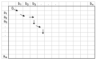
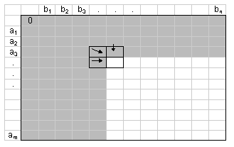
The second issue is about the iterative minimisation procedure. The discussion here will have to be schematic. Readers can find detailed and formal discussion of the algorithm in Waterman (1995), Sankoff and Kruskal (1983), or the documentation of the programs cited below. In general, given a finite state space S and two sequences a = (a1 ... am) and b = (b1 ... bn), where m is not equal to n, and the elements of a and b are drawn from S, the algorithm works by first creating a (m+1)×(n+1) matrix. To turn sequence a into sequence b from left to right is to move from the top left-hand cell of the matrix to the bottom right-hand cell (Figure 1). There are many paths one can take, but each path is built by a combination of moving down a row (which is equivalent to deleting the corresponding a element), moving right across a column (equivalent to inserting the corresponding b element), and moving diagonally (equivalent to making a substitution).
 |
 |
More importantly, it can be argued that the cluster identification problem is not an incidental issue traceable to cluster analysis. What OMA tries to do is to summarise what is potentially very complex sequence pattern with just one categorical variable -- the different sequence-types are the values of this variable. This should be reasonable in many situations, but perhaps not in all. In other words, it may be the case that in certain situations the sequences simply do not fall neatly into a clean typology. This is a cautionary note for potential OMA users.
Abbott, A. (1995) ‘Sequence Analysis: New Methods for Old Ideas’, Annual Review of Sociology, 21:93-113.
Abbott, A. and A. Hrycak (1990) ‘Measuring Resemblance in Sequence Analysis: An Optimal Matching Analysis of Musicians’ Careers’, American Journal of Sociology, 96:144-185.
Aldenderfer, M.S. and R.K. Blashfield (1984) Cluster Analysis, Newbury Park, Ca.: Sage.
Blossfeld, H-P., ed. (1995) The New Role of Women: Family Formation in Modern Societies, Boulder, CO.: Westview Press.
Blossfeld, H-P. and G. Rohwer (1995) Techniques of Event History Modeling, Mahwah, NJ: Lawrence Erlbaum.
Chan, T.W. (1995) ‘Optimal Matching Analysis: A Methodological Note on Studying Career Mobility’, Work and Occupations, 22:467-490.
Dale, A. and R.B. Davis, eds. (1994) Analyzing Social and Political Change: A Casebook of Methods, London: Sage.
Erikson, R. and J.H. Goldthorpe (1992) The Constant Flux: A Study of Class Mobility in Industrial Societies, Oxford: Clarendon Press.
Han, S-K. and P. Moen (1998) ‘Clocking Out: Multiplex Time in Retirement’, BLCC Working Paper #98-3, Cornell University.
Halpin, B. and T.W. Chan (1998) ‘Class Careers as Sequences: An Optimal Matching Analysis of Work-Life Histories’, European Sociological Review, 14:111-130.
Hogan, D.P. (1978) ‘The Variable Order of Events in the Life Course’, American Sociological Review, 43:573-586.
Sankoff, D and J.B. Kruskal, eds. (1983) Time Warps, String Edits, and Macro-Molecules: The Theory and Practice of Sequence Comparison, Reading: Addison-Wesley.
Stovel, K., M. Savage and P. Bearman (1996) ‘Ascription into Achievement: Models of Career Systems at Lloyds Bank, 1890-1970’, American Journal of Sociology, 102:358-399.
Waterman, M.S. (1995) Introduction to Computational Biology, London: Chapman and Hall.
Social Research Update is published by:
Department of Sociology
Telephone: +44 (0) 1 483 300800
Fax: +44 (0) 1 483 689551
Edited by Nigel Gilbert.
Spring 1999 © University of Surrey
Permission is granted to reproduce this issue of Social Research Update provided that no charge is made other than for the cost of reproduction and this panel acknowledging copyright is included with all copies.